Lecture-3: Overview
\(1-\phi\) and \(3-\phi\) Circuits & Quantities
Voltages and Currents in \(Y\) and \(\Delta\) Connections
\(Y \leftrightarrow \Delta\) conversion
Power in \(3-\phi\) circuits
\(3-\phi\)Circuits
Mostly electricity is generated by \(3-\phi\) AC generators
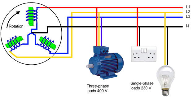
\(3-\phi\) system
has three phases, i.e., the current will pass through the three wires
there will be one neutral wire for passing the fault current to the earth ( \(3-\phi\) 4-wire system)
\(3-\phi\) system can be used as a \(1-\phi\) if one of their phase and the neutral wire is taken out from it
C.S.A of the neutral conductor is half of the live wire.
\(1-\phi\)System
\(3-\phi\)System

Why\(3-\phi\)is Preferred Over\(1-\phi\)?
Advantages of \(3-\phi\) over \(1-\phi\) system:
can be used as 3 \(\times\) \(1-\phi\) system
conductor needed is 75% of \(1-\phi\) circuit
instantaneous power in \(1-\phi\) system falls down to zero as can seen from the sinusoidal curve but in \(3-\phi\) the net power from all the phases gives a continuous power to the load.
higher efficiency and minimum losses
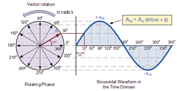
Phase Sequence, Line and Phase Quantities
Sinusoidal steady state and balanced condition \(\rightarrow\) 3-voltages are equal in magnitude and displaced by \(120^{\circ}\) w.r.t each other
Phase sequence: of voltage \(a-b-c\), where \(a\)-phase leads \(b\) by \(120^{\circ}\), \(b\) leads \(c\) by \(120^{\circ}\) and so on
Phase sequence applies to both time-domain and phasor-domain
Line Voltage: measured between any two line conductors
Phase Voltage: measured across any one component (source winding or load impedance)
Line current through any one line between a three-phase source and load
Phase current through any one component comprising a three-phase source or load.
\(3-\phi\) AC circuits are either \(Y\) or \(\Delta\) connected
Line/Phase and Load in\(3-\phi\)System
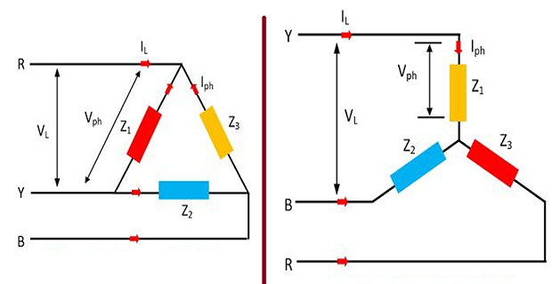
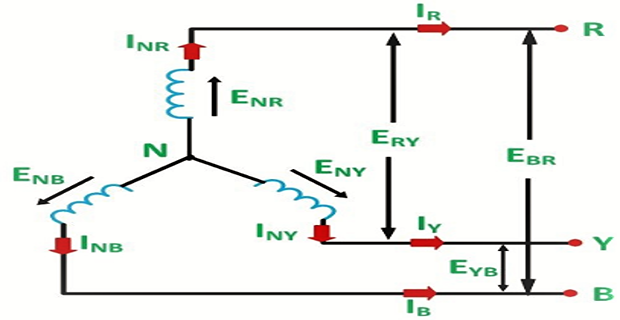
STAR (Y): Current & Voltage Relations
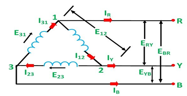
Delta(\(\Delta\)): Current & Voltage Relations
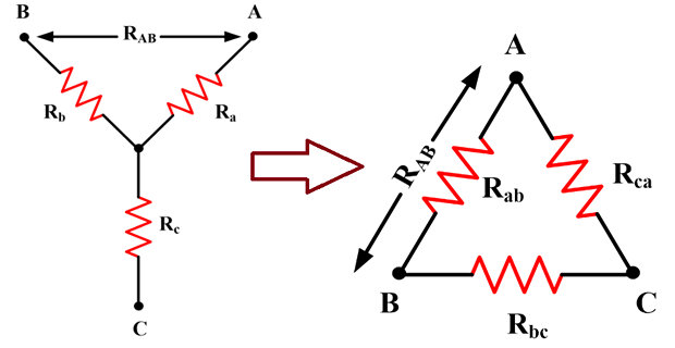
\(Y \leftrightarrow \Delta\)Transformation
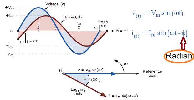
Power in 1-\(\phi\)and 3-\(\phi\)Circuits
- power equation 1-\[\mathrm{P}=\mathrm{VI} \cos \varphi\]
- power equation 3-\[\mathrm{P_{3\phi}}=3\mathrm{V_{ph}}\mathrm{I_{ph}} \cos \varphi\]
- \(3-\phi\)\[\begin{aligned} &P=3 \frac{V_{L}}{\sqrt{3}} I_{L} \operatorname{Cos} \varphi \\ \Rightarrow & \mathrm{P}=\sqrt{3} \mathrm{V}_{\mathrm{L}} \mathrm{I}_{\mathrm{L}} \operatorname{Cos} \varphi \end{aligned}\]
- \(\Delta\)\(3-\phi\)\[\begin{aligned} &\mathrm{P}=3 \mathrm{V}_{\mathrm{L}} \frac{\mathrm{I}_{\mathrm{L}}}{\sqrt{3}} \operatorname{Cos} \varphi\\ \Rightarrow & \sqrt{3} \mathrm{V}_{\mathrm{L}} \mathrm{I}_{\mathrm{L}} \cos \phi \end{aligned}\]
- Apparent Power\[\mathrm{P}_{\mathrm{a}}=\sqrt{3} \mathrm{V}_{\mathrm{L}} \mathrm{I}_{\mathrm{L}}\]
- Reactive Power\[P_{r}=\sqrt{3} V_{L} I_{L} \sin \varphi\]