Demonstrative Video
Introduction
Conductively-coupled: one loop affects the neighbouring loop through current conduction.
Magnetically-coupled: two loops with or without contacts between them affect each other through the magnetic field generated by one of them.
Current (ac or dc) flows through a conductor \(\Rightarrow\) magnetic field generated about the conductor.
Circuit context \(\Rightarrow\) magnetic flux (\(\phi\)) \(\Rightarrow\) \(B_n~(\text{Avg. normal component of flux-density}) \times A~ (\text{surface area of the loop})\)
When a time-varying \(\phi\) generated by one loop penetrates a second loop, a voltage is induced between the ends of the second wire
To distinguish Inductance (self inductance) \(\Rightarrow\) mutual-inductance
There is no such device as a “mutual inductor’’
Transformer basis of the concept of magnetic coupling.
Self and Mutual Inductance
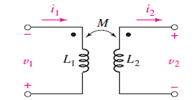
Mutual inductance: When two inductors (or coils) are in close proximity to each other, the magnetic flux caused by current in one coil links with the other coil, thereby inducing voltage in the latter.
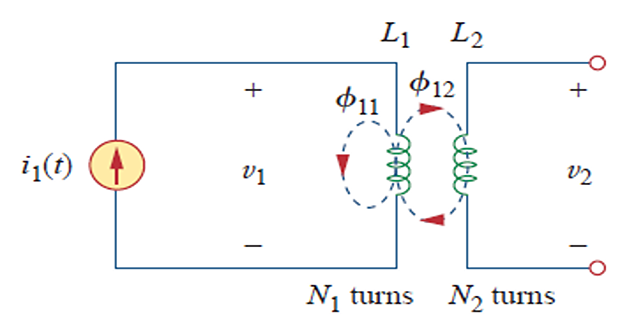
Mutual inductance diagram
M is also measured in henrys (H).
Mutual coupling only exists when the inductors or coils are in close proximity, and the circuits are driven by time-varying sources.
M is always a positive quantity but \(M \dfrac{di}{dt}\) can be \(\pm\)
Polarity of \(L \dfrac{di}{dt}\) is given by passive-sign convention but polarity of mutual voltage is not easy to determine due to 4-terminals involved.
Polarity determined by examining the physical orientation of both coils and applying Lenz’s law in conjunction with the right-hand rule
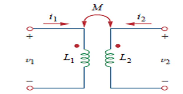
Dot Convention
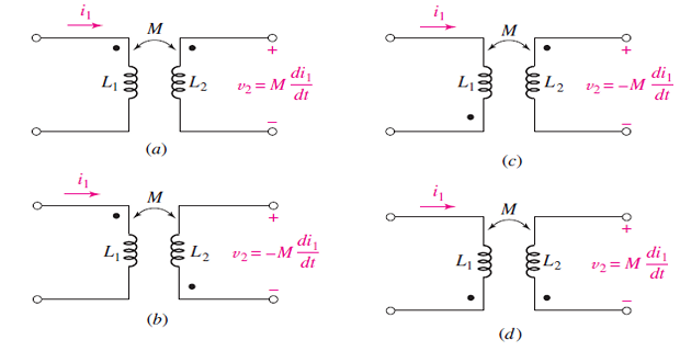
Dot convention diagram
A current entering the dotted terminal of one coil produces an open-circuit voltage with a positive voltage reference at the dotted terminal of the second coil.
A current entering the undotted terminal of one coil provides a voltage that is positively sensed at the undotted terminal of the second coil.
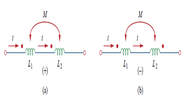
Series connection diagram
-
Series-aiding connection\[\boxed{L = L_1 + L_2 + 2M}\]
-
Series-opposing connection\[\boxed{L = L_1 + L_2 - 2M}\]
Combined Mutual and Self-Induction Voltage
Series-aiding connection
Series-opposing connection
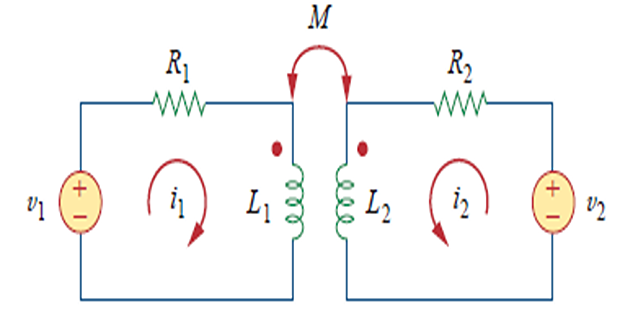
Circuit with resistors
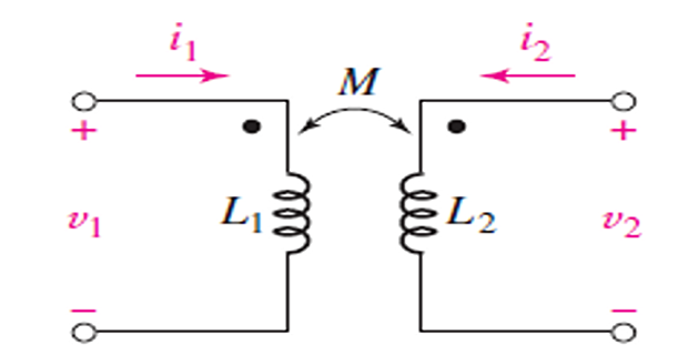
Energy in a Coupled Circuit
Assume \(i_1(0) = i_2(0) = 0\)
Energy in coupled circuit
-
maintaining from 0 to Increase\[\begin{aligned} p_{1}(t) &= v_{1} i_{1} = i_{1} L_{1} \frac{d i_{1}}{d t} \\ w_{1} &= \int p_{1} d t = L_{1} \int_{0}^{I_{1}} i_{1} d i_{1} = \frac{1}{2} L_{1} I_{1}^{2} \end{aligned}\]
-
from 0 to and increase Now maintain\[\begin{aligned} p_{2}(t) &= i_{1} M_{12} \frac{d i_{2}}{d t} + i_{2} v_{2} = I_{1} M_{12} \frac{d i_{2}}{d t} + i_{2} L_{2} \frac{d i_{2}}{d t} \\ w_{2} &= \int p_{2} d t = M_{12} I_{1} \int_{0}^{I_{2}} d i_{2} + L_{2} \int_{0}^{I_{2}} i_{2} d i_{2} \\ &= M_{12} I_{1} I_{2} + \frac{1}{2} L_{2} I_{2}^{2} \end{aligned}\]
-
have reached constant values and Total stored energy in coils when both\[w = w_1 + w_2 = \dfrac{1}{2} L_1 I_1^2 + \dfrac{1}{2} L_2 I_2^2 + M_{12} I_1 I_2\]
Equation derived assuming both coil currents entered the dotted terminals
-
If one current enters one dotted terminal while the other current leaves the other dotted terminal, the mutual voltage is negative\[w = w_1 + w_2 = \dfrac{1}{2} L_1 I_1^2 + \dfrac{1}{2} L_2 I_2^2 - M_{12} I_1 I_2\]
-
, which gives instantaneous energy stored and have arbitrary values they are replaced with and Since\[\boxed{w = \dfrac{1}{2} L_1 I_1^2 + \dfrac{1}{2} L_2 I_2^2 \pm M_{12} I_1 I_2}\]
What is the upper limit for the mutual inductance \(M\)?
-
Since the circuit is passive energy stored cannot be negative\[\begin{aligned} &\frac{1}{2} L_{1} i_{1}^{2} + \frac{1}{2} L_{2} i_{2}^{2} - M i_{1} i_{2} \geq 0 \\ \text{Completing square} \quad \Rightarrow &\frac{1}{2}\left(i_{1} \sqrt{L_{1}} - i_{2} \sqrt{L_{2}}\right)^{2} + i_{1} i_{2}\left(\sqrt{L_{1} L_{2}} - M\right) \geq 0 \\ \Rightarrow &\sqrt{L_{1} L_{2}} - M \geq 0 \\ \Rightarrow &M \leq \sqrt{L_{1} L_{2}} \\ \color{red}{\text{Coeff. of coupling}} \quad &k = \frac{M}{\sqrt{L_{1} L_{2}}} \\ &\boxed{M = k \sqrt{L_{1} L_{2}}} \quad 0 \leq k \leq 1 \text{ or } 0 \leq M \leq \sqrt{L_{1} L_{2}} \end{aligned}\]
\(M\) cannot be greater than the geometric mean of the self-inductances of the coils.
The extent to which \(M\) approaches the upper limit is specified by the coefficient of coupling.
Coupling Coefficient
The coupling coefficient is the fraction of the total flux emanating from one coil that links the other coil.
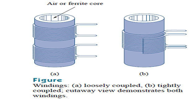
Coupling coefficient diagram
If the entire flux produced by one coil links another coil, then \(k=1\) and we have 100 percent coupling, or the coils are said to be perfectly-coupled.
For \(k < 0.5\) coils are said to be loosely coupled; and for \(k > 0.5\), they are said to be tightly coupled
Linear Transformer Coupled Circuits
Location of dots does not affect as \(M\) replaced with \(-M\)
Analysing magnetically coupled circuits is not easy or straightforward so sometimes convenient to replace it with an equivalent circuit with no magnetic coupling.
Elimination of Mutual Inductance
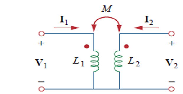
Actual transformer
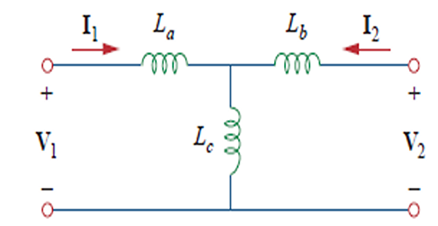
T-network
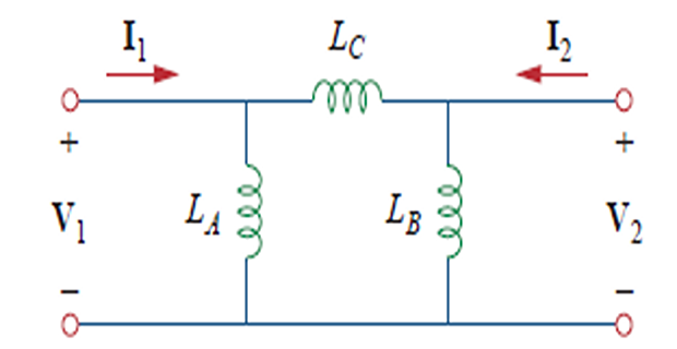
Pi-network